Using AWS Athena to query AWS service logs

Athena is a powerful tool for ad-hoc data analysis that may also be used as a log-querying engine. After all, logs are just data on S3! In this Gun.io blog post, Dustin Wilson explains how to use AWS Athena to query your service logs, illustrating with a sample configuration.

Introduction to Athena

In 2016, Amazon announced the release of Athena, a service that helps customers analyze data in S3 with standard SQL. Athena allows organizations to query volumes of structured and unstructured data without managing their own RDBMS, Presto, or Hadoop clusters. Athena shines when performing ad-hoc analysis on data sourced from multiple systems and when integrated with other AWS products (e.g. Glue, Quicksight, and LakeFormation). In the last few years, Amazon has introduced mechanisms to ensure ACID transactions, enforce row-level security, and integrate Athena with AWS’ machine learning ecosystem.

As a Data Engineer, I’ve primarily used Athena as a tool for ad-hoc queries on intermediate outputs from data pipelines. My teams have aimed to use Athena in such a way that analysts are able to build tables from data at (1), (2), or (3) and make suggestions on how we might formalize their analyses into scheduled data pipelines.

More recently, I’ve started using it to query logs from other AWS services (e.g. load balancers, DNS resolvers, or web firewalls). Analyzing my service logs with Athena has helped me answer questions like:

• Which IPs is my firewall denying access to most frequently?
• Is my load balancer using the most efficient algorithm to distribute traffic?
• Which of my application servers is receiving the highest number of HTTPS requests?

Functionally, using Athena as a log-querying engine is no different than using it for other ad-hoc data analysis. After all, logs are just data on S3! Since adopting this practice, I’ve found that Athena can be a powerful tool for debugging AWS services’ performance.

Properties of Athena

AWS markets Athena as a managed, serverless query service that allows users to analyze data with standard SQL. Before going through an example, we should discuss what each of those properties means and how Athena can improve on a more traditional data infrastructure.

• Managed — Under the hood, Athena uses Apache Presto, an open-source, parallel distributed query engine. For an infrastructure team, this means that there’s no longer the work of provisioning and managing a Presto cluster. While some knowledge of Presto could be helpful, getting started with Athena only requires data in S3 and knowledge of SQL.
• Serverless — Even with managed databases, teams still must properly size their databases and understand the load their queries will put on them. Estimating this incorrectly could lead to degraded query performance or an unexpectedly large bill. Because Athena is serverless and automatically scales workers to run in parallel, the risk associated with over or under provisioning databases is mitigated.
• ANSI SQL Compliant — Athena is based on Presto, so it inherits many of the properties that make Presto a popular choice for data teams. Among the most useful of these properties is Presto’s ability to use standard SQL to query a variety of different data sources. With Presto (and by extension, Athena), one can connect to HDFS, MySQL, Postgres, Cassandra, and many other data stores. Because SQL is well-known, Athena can enable analytics for more analysts and engineers who may not have knowledge of specific query languages.

A Sample Application and Configuring Athena 

AWS offers dozens of services that can be configured to write logs to Cloudwatch or S3. Until recently, I found it particularly difficult to debug services that logged exclusively to S3. For example, application load balancers (ALBs) write multiple files for each subnet every five minutes. When you’re trying to analyze patterns in system behavior, this format can be very unfriendly. Luckily, I could streamline this workflow with Athena, because ALBs write logs to S3.

For this demonstration, I’ll assume that you’re familiar with the basics of AWS Load Balancers and networking. This documentation on LBs and VPCs should provide enough background to follow the rest of the discussion.

Let’s imagine that we’ve set up a backend architecture that consists of the following:

• A containerized application, echo, that echos all incoming requests back to the user
• A VPC with a public and private subnet in each of two availability-zones
• Two EC2 instances running echo in the private subnets
• An internet-facing ALB in the public subnets

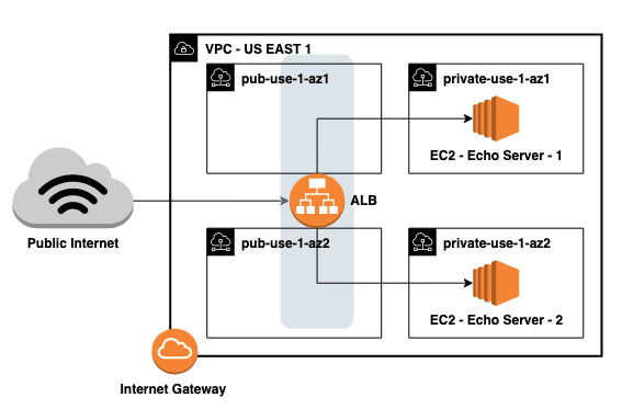
Given this architecture, logging ALB and VPC Flow (the logs between network interfaces in the VPC) could help us understand system performance or debug specific failed requests.

First, let’s navigate to the AWS Console and manually enable logging on this ALB by going to Actions > Edit Attributes.

The ALB console allows you to create a new S3 bucket with the correct permissions applied. If you’re interested in provisioning resources programmatically, you should be aware of the specific bucket policies this requires.

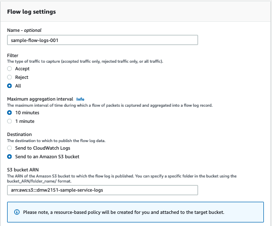
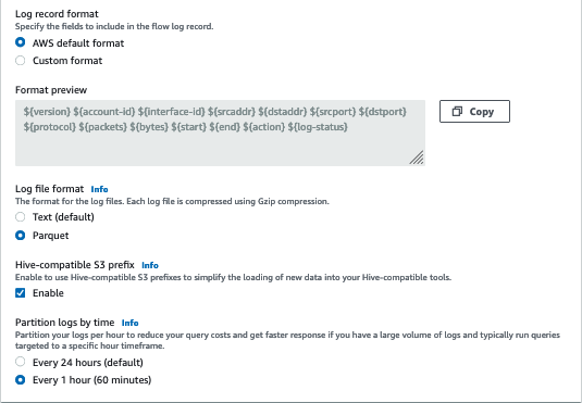
Let’s enable VPC Flow Logs as well. I can do that by navigating to the VPC console and clicking through Flow Logs > Create Flow Log. There are a lot of options on this page. I’ve been configuring my logs with the options shown below. I’ll highlight the reasons for these choices later on.

Finally, I can begin making requests to my ALB. Within 5 minutes, I can expect to see logs in the bucket specified in the previous step. Note that most AWS services write logs with a specific directory structure. In this case, your logs will be nested within a folder named AWSLogs.

I can download and inspect these logs manually, but the output is difficult to parse through. A single log entry will have a format similar to the example shown below:

h2 2018-07-02T22:23:00.186641Z app/my-loadbalancer/50dc6c495c0c9188
10.0.1.252:48160 10.0.0.66:9000 0.000 0.002 0.000 200 200 5 257
"GET https://10.0.2.105:773/ HTTP/2.0" "curl/7.46.0" ECDHE-RSA-AES128-GCM-SHA256 TLSv1.2
arn:aws:elasticloadbalancing:us-east-2:123456789012:targetgroup/my-targets/73e2d6bc24d8a067
"Root=1-58337327-72bd00b0343d75b906739c42" "-" "-"
1 2018-07-02T22:22:48.364000Z "redirect" "https://example.com:80/" "-" 10.0.0.66:9000 200 "-" "-"

Given that we’ll soon have thousands of these files containing millions of entries, we should probably develop a better strategy for analyzing them. If we configure a table in Athena, getting meaningful information from these files becomes much easier. I can navigate to the Athena console and run the following SQL to create a table from my ALB logs.

CREATE EXTERNAL TABLE IF NOT EXISTS alb_logs (
    type string,
    time string,
    elb string,
    client_ip string,
    client_port int,
    target_ip string,
    target_port int,
    request_processing_time double,
    target_processing_time double,
    response_processing_time double,
    elb_status_code int,
    target_status_code string,
    received_bytes bigint,
    sent_bytes bigint,
    request_verb string,
    request_url string,
    request_proto string,
    user_agent string,
    ssl_cipher string,
    ssl_protocol string,
    target_group_arn string,
    trace_id string,
    domain_name string,
    chosen_cert_arn string,
    matched_rule_priority string,
    request_creation_time string,
    actions_executed string,
    redirect_url string,
    lambda_error_reason string,
    target_port_list string,
    target_status_code_list string,
    classification string,
    classification_reason string
)

ROW FORMAT SERDE 'org.apache.hadoop.hive.serde2.RegexSerDe'
WITH SERDEPROPERTIES (
    'serialization.format' = '1', 'input.regex' = '([^ ]*) ([^ ]*) ([^ ]*) ([^ ]*):([0-9]*) ([^ ]*)[:-]([0-9]*) ([-.0-9]*) ([-.0-9]*) ([-.0-9]*) (|[-0-9]*) (-|[-0-9]*) ([-0-9]*) ([-0-9]*) \"([^ ]*) (.*) (- |[^ ]*)\" \"([^\"]*)\" ([A-Z0-9-_]+) ([A-Za-z0-9.-]*) ([^ ]*) \"([^\"]*)\" \"([^\"]*)\" \"([^\"]*)\" ([-.0-9]*) ([^ ]*) \"([^\"]*)\" \"([^\"]*)\" \"([^ ]*)\" \"([^\s]+?)\" \"([^\s]+)\" \"([^ ]*)\" \"([^ ]*)\"'
) LOCATION 's3://${bucket_name}/AWSLogs/${aws_account_id}/elasticloadbalancing/${region_slug}';

From here, no further configuration is needed! At this point, you can begin writing SQL against your service logs. There are many choices you could make to have those queries run faster and be less expensive, but let’s work on an applied example with a small dataset before diving into questions of performance and optimization.

Debugging a Sample Incident

Now that we have a table that contains a log of all requests to the load balancer, we can start to develop hypotheses around our service’s performance. For example, we may want to know if all application hosts are serving responses with similar latency. Using the query below, we calculate the average response time by host within the last 15 minutes.

At steady-state, it seems that they’re roughly equal. Let’s say a developer accidentally pushes a configuration that causes the response time of the application to spike. Looking at only the ALB dashboard, we can observe the change in performance, but we can’t see any additional details about the incident.

Because we have ALB logs at our fingertips, we might re-use the query from above to check if the slowdown is affecting all hosts equally.

From this output, we can determine that not all hosts are affected! The responses sent to 10.0.3.9are completing as expected, while those sent to 10.0.4.31 are taking over 200ms. In this case, Athena helped us precisely identify the affected resources and gave us the ability to generate metrics that are more precise than the default service metrics.

Improving Query Performance

This is a nice use-case, but it neglects a lot of the nuance of querying data in S3. As we get more data, these queries will become slow and expensive. Athena billing is based on the total data scanned by your queries ($5/TB), so it’s in our best interest to structure files in a way that minimizes data scanned. The most effective ways to do this are:

• Columnar Formats – Columnar formats like Parquet and ORC allow Athena to scan only the columns that the query references. With well designed queries, this can lead to less data scanned and lower costs.
• Compressed Formats – Queries over files in compressed data formats (e.g. *.csv.gz vs .csv) are less expensive because less data is stored (S3 charges) and scanned (Athena charges).
• Splittable Formats – Athena can split single files of certain formats onto multiple reader nodes, and this can lead to faster query results.
• Partitioning Tables – Partitioning divides your table based on values such as date, AWS account, AWS region, etc. Given a query referencing specific partitions, Athena will only scan the relevant files. If a column often appears in a WHERE clause, it may be a candidate for a partition column.

These elements of file and table management can add additional complexity, but they can also yield orders of magnitude improvement in query performance and cost. To demonstrate how these properties can be used to improve performance, let’s return to the VPC logs we created earlier.

A Brief Look at Parquet Logs

When we created VPC logs, we elected to create them as automatically-partitioned parquet files. The advantages of this format should be clear conceptually, but let’s examine a few queries to demonstrate how much less data can be scanned with a properly designed data file structure and table format.

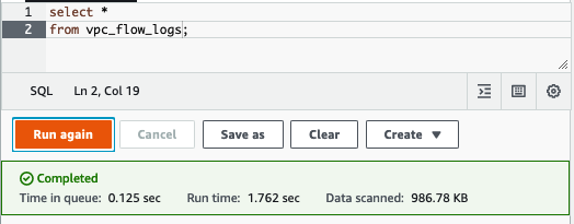
As with ALB logs, I used a CREATE EXTERNAL TABLE statement to create a table in Athena partitioned by date and hour. The AWS VPC logs documentation provides a detailed example for defining partitions on parquet files. In the following query, Athena does a full scan on all the VPC Flow logs created by our system. It’s just under 1MB.

What if instead of accessing all the data from this table, we were only interested in a small window? With a non-partitioned table, Athena would scan all log files. Because the table is partitioned by hour, writing a query like the one below leads Athena to only scan files in /hour=02. Instead of scanning the full 1MB, this query only scanned about 200KB.

Finally, let’s look at an example where we’re interested in a subset of columns. Because the data is stored in a columnar format, and the query only refers to single column bytes, Athena only scans a single column. This change leads to a further reduction in data scanned from 200KB to just 25KB.

It’s important to remember that this last query would still scan the full 988KB if our table was structured inefficiently. Although these volumes are small, the ratios (and pricing) hold as we scale up. On tables that are hundreds of GB, structuring your Athena tables well can end up saving hundreds (or thousands) of dollars. For organizations that are heavily invested in Athena, it’s a common strategy to run an ETL job that partitions tables and converts *.log.gzto *.parquet files.

Final Notes 

Athena can be a powerful tool for ad-hoc data analysis. I’ve found that with a good understanding of service logs and the right table structure, it can also be a tool for quickly and efficiently understanding your system’s performance and health.